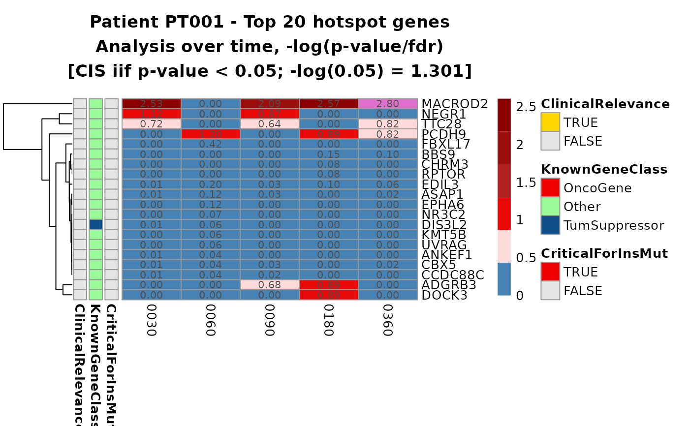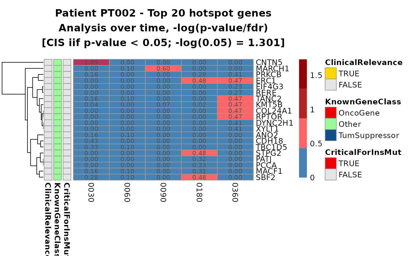
Heatmaps for the top N common insertion sites over time.

This function computes the visualization of the results of the function CIS_grubbs_overtime() in the form of heatmaps for the top N selected genes over time.

Usage

top_cis_overtime_heatmap(
  x,
  n_genes = 20,
  timepoint_col = "TimePoint",
  group_col = "group",
  onco_db_file = "proto_oncogenes",
  tumor_suppressors_db_file = "tumor_suppressors",
  species = "human",
  known_onco = known_clinical_oncogenes(),
  suspicious_genes = clinical_relevant_suspicious_genes(),
  significance_threshold = 0.05,
  plot_values = c("minus_log_p", "p"),
  p_value_correction = c("fdr", "bonferroni"),
  prune_tp_treshold = 20,
  gene_selection_param = c("trimmed", "n", "mean", "sd", "median", "mad", "min", "max"),
  fill_0_selection = TRUE,
  fill_NA_in_heatmap = FALSE,
  heatmap_color_palette = "default",
  title_generator = NULL,
  save_as_files = FALSE,
  files_format = c("pdf", "png", "tiff", "bmp", "jpg"),
  folder_path = NULL,
  ...
)

Arguments

x: Output of the function CIS_grubbs_overtime(), either in single data frame form or nested lists
n_genes: Number of top genes to consider
timepoint_col: The name of the time point column in x
group_col: The name of the group column in x
onco_db_file: Uniprot file for proto-oncogenes (see details). If different from default, should be supplied as a path to a file.
tumor_suppressors_db_file: Uniprot file for tumor-suppressor genes. If different from default, should be supplied as a path to a file.
species: One between "human", "mouse" and "all"
known_onco: Data frame with known oncogenes. See details.
suspicious_genes: Data frame with clinical relevant suspicious genes. See details.
significance_threshold: The significance threshold
plot_values: Which kind of values should be plotted? Can either be "p" for the p-value or "minus_log_p" for a scaled p-value of the Grubbs test
p_value_correction: One among "bonferroni" and "fdr"
prune_tp_treshold: Minimum number of genes to retain a time point. See details.
gene_selection_param: The descriptive statistic measure to decide which genes to plot, possible choices are "trimmed", "n", "mean", "sd", "median","mad", "min", "max". See details.
fill_0_selection: Fill NA values with 0s before computing statistics for each gene? (TRUE/FALSE)
fill_NA_in_heatmap: Fill NA values with 0 when plotting the heatmap? (TRUE/FALSE)
heatmap_color_palette: Colors for values in the heatmaps, either "default" or a function producing a color palette, obtainable via grDevices::colorRampPalette.
title_generator: Either NULL or a function. See details.
save_as_files: Should heatmaps be saved to files on disk? (TRUE/FALSE)
files_format: The extension of the files produced, supported formats are "pdf", "png", "tiff", "bmp", "jpg". Relevant only if files_format = TRUE
folder_path: Path to the folder where files will be saved
...: Other params to pass to pheatmap::pheatmap

Value

Either a list of graphical objects or a list of paths where plots were saved

Details

Oncogene and tumor suppressor genes files

These files are included in the package for user convenience and are simply UniProt files with gene annotations for human and mouse. For more details on how this files were generated use the help ?tumor_suppressors, ?proto_oncogenes

Known oncogenes

The default values are included in this package and it can be accessed by doing:

If the user wants to change this parameter the input data frame must preserve the column structure. The same goes for the suspicious_genes parameter (DOIReference column is optional):

Top N gene selection

Since the genes present in different time point slices are likely different, the decision process to select the final top N genes to represent in the heatmap follows this logic:

Each time point slice is arranged either in ascending order (if we want to plot the p-value) or in descending order (if we want to plot the scaled p-value) and the top n genes are selected
A series of statistics are computed over the union set of genes on ALL time points (min, max, mean, ...)
A decision is taken by considering the ordered gene_selection_param (order depends once again if the values are scaled or not), and the first N genes are selected for plotting.

Filling NA values prior calculations

It is possible to fill NA values (aka missing combinations of GENE/TP) with 0s prior computing the descriptive statistics on which gene selection is based. Please keep in mind that this has an impact on the final result, since for computing metrics such as the mean, NA values are usually removed, decreasing the overall number of values considered - this does not hold when NA values are substituted with 0s.

The statistics

Statistics are computed for each gene over all time points of each group. More in detail, n: counts the number of instances (rows) in which the genes appears, aka it counts the time points in which the gene is present. NOTE: if fill_0_selection option is set to TRUE this value will be equal for all genes! All other statistics as per the argument gene_selection_param map to the corresponding R functions with the exception of trimmed which is a simple call to the mean function with the argument trimmed = 0.1.

Aesthetics

It is possible to customise the appearence of the plot through different parameters.

fill_NA_in_heatmap tells the function whether missing combinations of GENE/TP should be plotted as NA or filled with a value (1 if p-value, 0 if scaled p-value)
A title generator function can be provided to dynamically create a title for the plots: the function can accept two positional arguments for the group identifier and the number of selected genes respectively. If one or none of the arguments are of interest, they can be absorbed with ....
heatmap_color_palette can be used to specify a function from which colors are sampled (refers to the colors of values only)
To change the colors associated with annotations instead, use the argument annotation_colors of pheatmap::pheatmap() - it must be set to a list with this format:

list(
  KnownGeneClass = c("OncoGene" = color_spec,
                     "Other" = color_spec,
                     "TumSuppressor" = color_spec),
  ClinicalRelevance = c("TRUE" = color_spec,
                        "FALSE" = color_spec),
  CriticalForInsMut = c("TRUE" = color_spec,
                        "FALSE" = color_spec)
)

Examples

data("integration_matrices", package = "ISAnalytics")
data("association_file", package = "ISAnalytics")
aggreg <- aggregate_values_by_key(
    x = integration_matrices,
    association_file = association_file,
    value_cols = c("seqCount", "fragmentEstimate")
)
cis_overtime <- CIS_grubbs_overtime(aggreg)
#> Warning: Warning: missing genes in refgenes table
#> ℹ A total of 5 genes were found in the input data but not in the refgene table. This may be caused by a mismatch in the annotation phase of the matrix. Here is a summary: 
#> # A tibble: 5 × 3
#>   GeneName  GeneStrand chr  
#>   <chr>     <chr>      <chr>
#> 1 PLEKHG4B  -          14   
#> 2 CRELD2    -          15   
#> 3 UBE2D2    +          16   
#> 4 LINC01133 +          19   
#> 5 HTR4      +          6    
#> ℹ NOTE: missing genes will be removed from the final output! Review results carefully
#> ℹ A total of 25 IS will be removed because of missing genes ( 2.33 % of total IS in input)
hmaps <- top_cis_overtime_heatmap(cis_overtime$cis,
    fill_NA_in_heatmap = TRUE
)
#> Loading annotated genes -  species selected: 
#> • Homo sapiens (Human)
#> Loading annotated genes -  done



# To re-plot:
# grid::grid.newpage()
# grid::grid.draw(hmaps$PT001$gtable)